The Architecture of Execution — ICT Trading Models

Introduction to ICT Trading Models & Setups

In the Inner Circle Trader (ICT) methodology, the difference between merely understanding market theory and successfully trading the market comes down to one crucial bridge: the model. While core concepts such as liquidity, displacement, Fair Value Gaps (FVGs), order blocks, and inducements form the permanent grammar of price movement, models are the practical, repeatable arrangements of those concepts that traders use to enter, manage, and complete trades. Concepts teach you what the market is doing; models teach you when to act. This distinction is the heart of execution. Unlike the core concepts, which remain true across every timeframe and asset class, models are highly contextual. They emerge only under specific combinations of liquidity positioning, session timing, volatility profiles, and structural alignment. They are not signals but narrative sequences. Each model is a storyline composed of familiar components—a liquidity grab, a displacement, a retracement, and a confirmation. What changes from one model to another is not the building blocks themselves, but the order in which those blocks appear and the environment in which they manifest.

ICT models exist to solve the practical problem every trader faces: identifying high-probability moments in a constantly moving market. Even with a perfect understanding of individual concepts, a trader needs a way to organize them into predictable, executable sequences. A liquidity sweep by itself means nothing unless it is paired with the right displacement. A Fair Value Gap is just an imbalance unless it appears inside a larger narrative. An Order Block can form at any time, but only specific ones matter. Models dictate which concepts are relevant at a specific moment and what should logically follow. They distill the infinite complexity of price action into a small number of recognizable patterns that reflect institutional behavior. Every ICT model is built on a universal storyline: liquidity is engineered, liquidity is taken, institutional displacement confirms intent, price retraces to rebalance, a protected entry zone forms, and the market delivers toward the draw on liquidity.

This chapter is designed to move the trader from theory to execution. Each model presented hereafter is a narrative structure—not a rigid rulebook, but a consistent script that institutions follow when executing large orders. You will learn how models adapt across sessions, how to recognize them forming in real time, and how to validate them using displacement and Market Structure Shifts. By mastering these models, you stop hunting for random entries and start following the structured scripts that institutions have been repeating for decades. The market stops appearing chaotic and begins to read like chapters within a familiar story.

Chapter 1 — The Liquidity Sweep Reversal Model

“Raid → Shift → Retrace → Deliver”

Introduction: The Blueprint of Institutional Reversals

The Liquidity Sweep Reversal serves as the single most critical model within the entire Inner Circle Trader framework and forms the backbone of the 2022 Mentorship Model. It is not merely a chart pattern, but the purest expression of institutional behavior, repeating consistently across every asset class, timeframe, market condition, and trading session. This model represents the internal mechanics of how price transitions from a state of manipulation to genuine delivery. If there is a singular "Holy Grail" setup that captures the essence of Smart Money Concepts—a repeatable structure capable of forming the basis of an entire professional career—it is this specific sequence. Fundamentally, the concept relies on the principle that before price can move in its true, intended direction, it must first move in the opposing direction. This counter-intuitive movement is intentional, engineered to create traps, harvest liquidity, fill large institutional orders, and mislead retail traders before the market aligns with the daily bias.

Underneath this apparent simplicity lies a deeply structured sequence that defines the anatomy of a trade. The process begins with a clear daily bias determined from higher timeframe charts, followed by the identification of a liquidity pool resting opposite that bias. The market then executes a deliberate raid or sweep into that pool, followed by a violent rejection that indicates institutional accumulation. This rejection must be backed by displacement, leading to a confirmed Market Structure Shift (MSS). Finally, the price retraces into a precision PD array—such as a Fair Value Gap (FVG) or Order Block—before executing a clean delivery toward the higher-timeframe draw. The brilliance of this model stems from the insight that institutions do not chase price; they create the specific conditions they require. Because they cannot move massive capital without triggering volatility, they must manufacture liquidity first to avoid slippage.

Part 1 — The Logic Begins With Daily Bias

A liquidity sweep reversal cannot be traded in a vacuum; its success is entirely dependent on the higher-timeframe narrative. The analysis must always begin with determining which side of the market price is most likely to be drawn toward for the day. This daily bias is derived from a synthesis of weekly and daily swing points, unfilled Fair Value Gaps on higher timeframe charts, massive Order Blocks or Breaker Blocks, and prior highs or lows. The purpose of establishing a daily bias is not strictly prediction, but rather orientation, identifying the most likely "draw on liquidity" for the session. For instance, if the higher-timeframe structure is bullish and a cluster of equal highs sits above the current price, the market is magnetized upward. Conversely, if the structure is bearish and a deep pocket of Sell-Side Liquidity exists below, the market is magnetized downward. This directional magnet provides the trader with a governing framework: on a long day, price seeks buy-side liquidity later, but will often run sell-side liquidity first. On a short day, price seeks sell-side liquidity later, but often runs buy-side liquidity first. The essential principle here is that before the market reaches its higher-timeframe target, it must take out the opposing intrinsic liquidity.

Part 2 — Identifying the Liquidity That Must Be Raided

Once the daily bias indicates the true target, the trader must identify what liquidity stands in the way. Price cannot simply travel to the target; it requires fuel to get there. This fuel comes in two main categories: Buy-Side Liquidity (BSL) and Sell-Side Liquidity (SSL). Buy-Side Liquidity rests above previous swing highs, equal highs, trendline highs, and session highs from Asia or London. This liquidity is generated by short stop-losses (market buy orders) and breakout buy-stops. Sell-Side Liquidity rests below previous swing lows, equal lows, trendline lows, and session lows. This liquidity is generated by long stop-losses (market sell orders) and breakout sell-stops. The sweep reversal model invariably begins by attacking one of these zones. Crucially, the zone swept is the one located opposite the daily bias. On a bullish day, the market will sweep Sell-Side Liquidity first to accumulate long positions. On a bearish day, the market will sweep Buy-Side Liquidity first to accumulate short positions. This creates a "wrong-direction move" that retail traders often confuse with a breakout. While the retail trader sees a breakout and attempts to join the momentum, the institutional trader sees a stop raid designed to fill positions.

Part 3 — The Raid: The Manipulation Leg

The liquidity sweep, or the raid, is the intentional movement into an obvious liquidity pool. Visually, this is characterized by a sharp spike beyond a prior high or low, a wick piercing a clear liquidity level, or a fast acceleration into the pool followed by a brief candle body close beyond the level. Psychologically, this represents the discrepancy between the retail view and institutional reality. Retail traders, seeing the rapid movement, often believe a genuine breakout is occurring and jump into the trade. However, the institutional reality is that this breakout exists solely to fill their orders. The raid is the institutional solution to the problem of liquidity. To trade significant size, they require counterparties, and retail traders unknowingly supply this by placing stops in predictable locations. During the raid, longs are stopped out, shorts are stopped in, and momentum traders are baited, creating massive counterparty flow. For example, on a bullish day, institutions need sellers to buy from. These sellers are found below previous lows where long stop-losses rest. By driving price down quickly, institutions trigger these stops, creating massive sell orders which the institutions then buy. This process is the "Accumulation via Manipulation" stage.

Part 4 — Displacement: The Institutional Signature

Following the sweep of liquidity, the market must prove that the move was an intentional trap rather than a genuine breakout. This confirmation is provided by displacement, which serves as the "footprint" of institutional sponsorship. Displacement manifests as a sudden, violent rejection wick after the raid, followed by a series of large, directional candles with minimal wicks in the direction of delivery. This "one-sided" push indicates urgency and verifies that the initial sweep was indeed a trap; if the breakout had been genuine, price would have continued through the level rather than snapping back. Displacement serves three critical purposes: it confirms the trap, it breaks internal market structure (CHoCH), and it creates PD arrays such as Fair Value Gaps (FVGs) and Order Blocks (OBs). These arrays are essential as they form the foundation for the subsequent retracement entry. Without the presence of displacement, a sweep is meaningless, as every chart contains sweeps; only displacement imbues them with legitimacy and tradeability.

Part 5 — Market Structure Shift (MSS): The Reversal Confirmation

Displacement alone is not the signal; the Market Structure Shift (MSS) provides the necessary confirmation. An MSS occurs when the displacement leg breaks a significant internal swing point that represents the last line of defense for the old trend. This break must happen via a displacement candle, signaling that the old trend is terminated and a new one has begun. A valid MSS must be decisive, backed by displacement, break a meaningful swing, and align with the daily bias. Once the MSS occurs, the trader's bias shifts immediately. If the MSS is bullish, the trader looks exclusively for longs; if bearish, they look exclusively for shorts. The occurrence of the MSS transitions the trader’s state from passive observation to active preparation. It marks the shift from watching and waiting to targeting specific levels and planning the entry.

Part 6 — The Retracement: Returning to the Origin of Displacement

After the displacement and the Market Structure Shift, price must retrace. Institutions do not chase price; they allow it to return to a zone where they have left unfilled orders. Price almost always retraces into a high-probability PD Array, such as a Fair Value Gap, which is the most common entry point; an Order Block, which is the origin of the displacement; or a Balanced Price Range or Breaker Block. To validate the retracement, traders must apply valuation concepts. For a bullish retracement, price must pull back into a Discount marketplace (below 50% of the range). For a bearish retracement, price must pull back into a Premium marketplace (above 50% of the range). Precision is further refined using the Optimal Trade Entry (OTE) zone, generally between the 61.8% and 79% retracement levels. The perfect scenario for entry combines the initial sweep, the MSS, strong displacement, a clear PD array, alignment with Discount/Premium zones, and specific "kill zone" timing. This confluence creates the highest probability setup.

Part 7 — Delivery: The Move Toward the Higher-Timeframe Target

Once the retracement is complete and the entry is filled, the market enters the delivery phase. This phase is characterized by clean displacement pushes, consistent market structure (higher highs and higher lows for longs; lower highs and lower lows for shorts), minimal deep pullbacks, and orderly mitigation. The price moves toward the higher-timeframe draw identified during the daily bias analysis. Common targets for delivery include the opposite side of the Asian range, London highs or lows, the previous day's high or low, higher-timeframe FVGs or Order Blocks, and liquidity voids. This delivery completes the cycle of "Raid → Shift → Retrace → Deliver," fulfilling the skeleton of the price movement.

Part 8 — Why This Model Works Across All Markets and Timeframes

The Liquidity Sweep Reversal is universally applicable because it addresses the fundamental necessities of market mechanics. All markets, whether crypto, forex, indices, or stocks, require liquidity to function, and retail traders predictably place stops in obvious locations like equal highs or trendlines. Professional liquidity providers exploit this predictability, utilizing the sweep to access the liquidity they need to fill large orders. Furthermore, institutions must disguise their intent, using the raid to hide accumulation or distribution. The subsequent Market Structure Shift and displacement reveal the true intent that can no longer be hidden, while the retracement offers high-probability entries where institutional orders remain. Finally, delivery follows the path to where the remaining liquidity resides. This model is not a trick or a temporary anomaly; it is the unavoidable microstructure of markets dominated by large players.

Chapter 2 — Power of Three, Asia Range & Daily Profiles

“The Full Daily Narrative: Accumulation → Manipulation → Distribution”

Introduction: The Anatomy of the Daily Candle

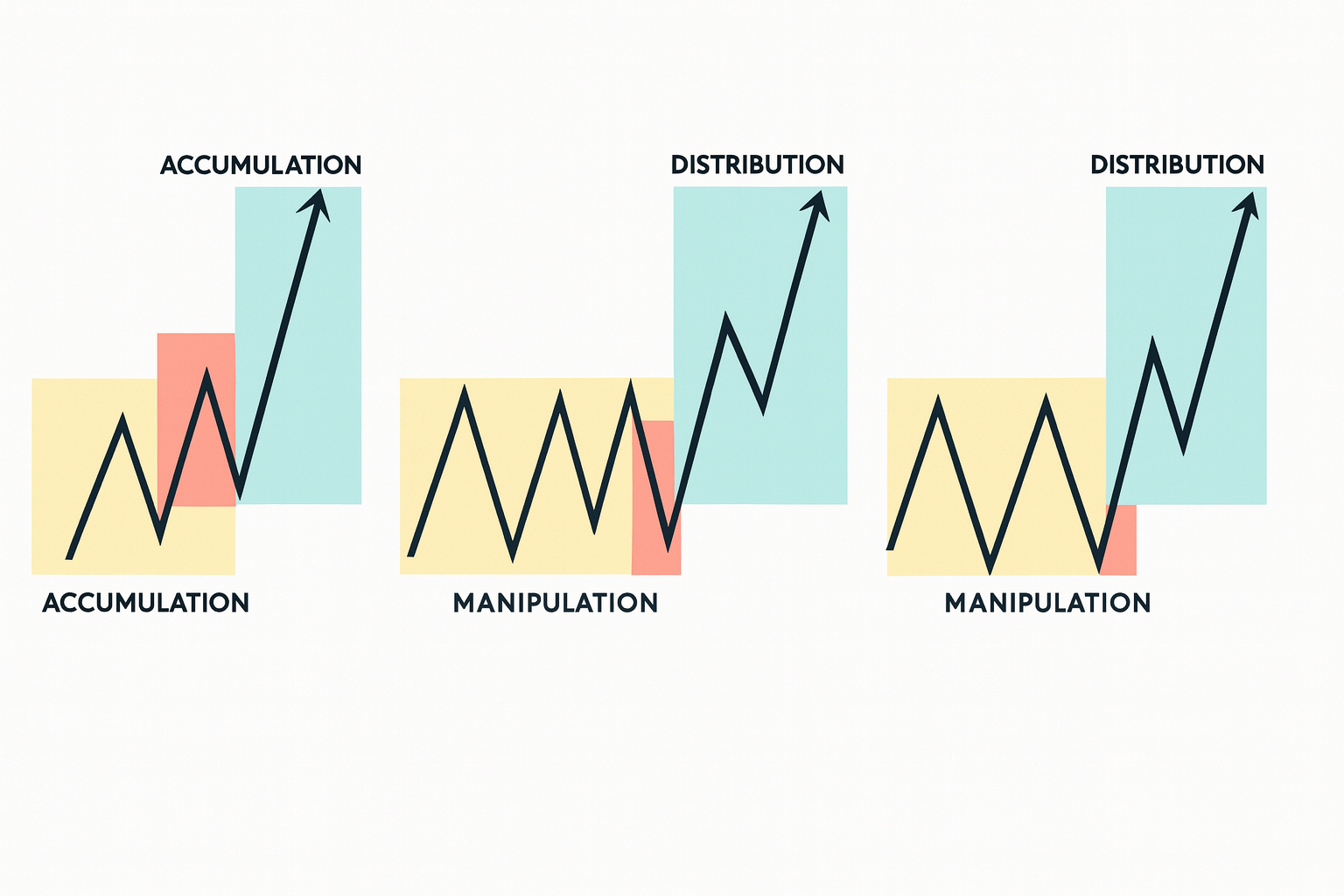
The Power of Three (AMD) is the overarching narrative framework that explains how a daily candle is constructed. It asserts that every trading day undergoes a cyclical metamorphosis through three distinct phases: Accumulation, Manipulation, and Distribution. This concept dictates that the Open, High, Low, and Close (OHLC) of a daily candle are not random data points, but the result of a deliberate engineering process. This model transforms the randomness of intraday trading into a coherent structure by recognizing that the daily price action is a story written by institutional algorithms, designed to facilitate the transfer of assets.

The essential principle of the Power of Three aligns with the formation of any daily candle: on a bullish day, the candle must open, drop (to form the low/manipulation), and then rise (distribution) to close. The drop below the open is the necessary manipulation needed to secure optimal pricing.

Part 1: Accumulation — The Staging Ground (Asia)

The narrative begins with Accumulation. This phase typically occurs during the Asian Session (20:00 to 00:00 New York time), where low volatility leads to price compression. The market oscillates within a narrow Asian Range, and institutions use this dormancy to build large positions and, crucially, to engineer liquidity at the range boundaries (Buy-Side Liquidity above the Asian High, Sell-Side Liquidity below the Asian Low). To the institutional trader, the Asian Range is the quiet staging ground where the initial conditions for the day’s volatility are set.

The Asian Range provides the necessary context for the day’s structure. The trader determines the Daily Bias from higher timeframes and anticipates the relationship: on a bullish day, the algorithm is expected to drive price below the Asian Low to secure cheap buy orders; on a bearish day, price will drive above the Asian High to secure expensive sell orders.

Part 2: Manipulation — The Judas Swing

As the London Open Kill Zone approaches (typically 02:00 to 05:00 New York time), the market transitions to Manipulation. This is expressed through the Judas Swing: a sudden, forceful run beyond the boundaries of the Asian Range. This deceptive price thrust is designed to trick retail traders into believing a breakout has occurred, simultaneously stopping out early buyers/sellers and luring breakout traders.

The Judas Swing performs two critical functions:

Liquidity Harvest: It violently breaks the opposing liquidity pool (e.g., raiding Sell-Side Liquidity below the Asian Low on a bullish day), providing the buy-side volume institutions need to fill their large orders.
Profile Formation: It establishes the High of the Day or the Low of the Day, forming the wick of the daily candle.

Following the raid, the market must confirm the manipulation is complete via displacement and a Market Structure Shift (MSS) back in the direction of the true daily bias. This signals that the trap has been sprung and the true trend is about to begin. The trader then looks for a retracement entry (often an Optimal Trade Entry (OTE) or Fair Value Gap) aligned with the heavy institutional flow initiated at the manipulation low/high.

Part 3: Distribution — The Delivery and Day Profiles

The final phase is Distribution. Having secured optimal pricing during the manipulation, the smart money now drives price toward the true higher-timeframe draw on liquidity. This is the expansion leg, forming the long "body" of the daily candle. This move often stretches across the remainder of the London session and into the New York Open, characterized by clean, directional pushes.

Understanding the Power of Three allows traders to categorize trading days into recurring Day Profiles. These templates describe the expected sequence of OHLC formation:

The Classic Buy Day (OLHC): Price opens, drops (manipulation/Judas Swing) to form the Low of the Day (L), and then extends violently upward to form the High of the Day (H) and closes near the highs (C).
The Classic Sell Day (OHLC): Price opens, rallies (manipulation/Judas Swing) to form the High of the Day (H), and then extends violently downward to form the Low of the Day (L) and closes near the lows (C).
The London Reversal: The manipulation extends through much of the London session, and the true distribution and reversal do not occur until the New York Open.
The Consolidation Day: The Power of Three fails to expand, with accumulation dominating the entire session, typically ahead of major news events.

By adopting the AMD narrative, the trader gains the overarching canvas for understanding all other models; the Silver Bullet is simply a time-specific execution within the distribution phase, and the Liquidity Sweep Reversal is the structural pivot from manipulation to distribution.

Chapter 3 — The Silver Bullet Model

“Time-Boxed Intraday Liquidity + FVG Delivery”

Introduction: Precision Through Temporal Constraint

While the Liquidity Sweep Reversal provides the structural backbone of institutional trading, and the Asia Range Model provides the daily narrative arc, the Silver Bullet Model represents the pinnacle of temporal precision. It is one of the most widely adopted strategies within the Inner Circle Trader (ICT) methodology precisely because it eliminates the variable of "randomness" by strictly limiting the trader’s engagement to specific, recurring 60-minute intervals. This model is not merely a setup; it is a recognition of the algorithmic "macros"—automated sub-routines within the market-making algorithm that execute specifically to reprice assets during key transitional periods of the day.

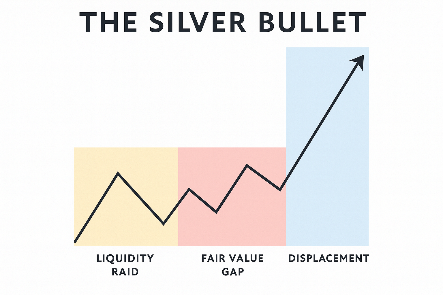
The Silver Bullet distills the complex ICT framework into its most compact and executable form: a liquidity raid, a displacement, and a Fair Value Gap (FVG) entry, all occurring within a rigid time constraint. By forcing the trader to focus only on these specific windows, the model removes the paralysis of analysis that comes from watching every price tick. It posits that Time is more important than Price. If you are in the right time window, the price action becomes predictable; outside of these windows, price action is often merely noise or accumulation.

Part 1: The Three Algorithmic Windows

The core of the Silver Bullet is the specific timing of the "Macros." These are not arbitrary hours; they are the periods where the interbank algorithm is programmed to seek liquidity and rebalance inefficiencies as one session hands off to another or as a session seeks to resolve its daily range. There are three distinct Silver Bullet windows every trading day (all times in Eastern Standard Time/New York Time):

The London Silver Bullet (03:00 AM – 04:00 AM) This window occurs in the heart of the London session. It typically capitalizes on the liquidity generated after the initial London Open (02:00 AM) volatility. By 3:00 AM, the initial "Judas Swing" has often completed, and the market is looking to expand toward the session's true mid-term objective. This window offers high-probability continuations of the move established at the London Open.
The New York AM Silver Bullet (10:00 AM – 11:00 AM) This is the most popular and highly traded window. It begins immediately after the "New York Open Kill Zone" (07:00–10:00 AM) concludes and after major economic news (often released at 8:30 AM or 10:00 AM) has unsettled the market. The 10:00 AM macro is designed to settle the initial volatility and typically creates a clean run toward the "lunch hour" liquidity. It is famous for providing clear, one-sided delivery.
The New York PM Silver Bullet (02:00 PM – 03:00 PM) As the market approaches the daily close, the afternoon macro engages to reprice the asset for the end of the day. This window often sees the market seeking to "close in" on a target, such as an unfilled gap or an exposed high/low, before the final bell. It provides the last clean opportunity for intraday liquidity delivery.

Part 2: The Anatomy of the Setup

Unlike broader narrative models that require tracking daily bias or weekly profiles, the Silver Bullet is a self-contained microstructure. However, it strictly adheres to the laws of institutional order flow. The setup must materialize within the hour. If the components do not align during the window, there is no trade.

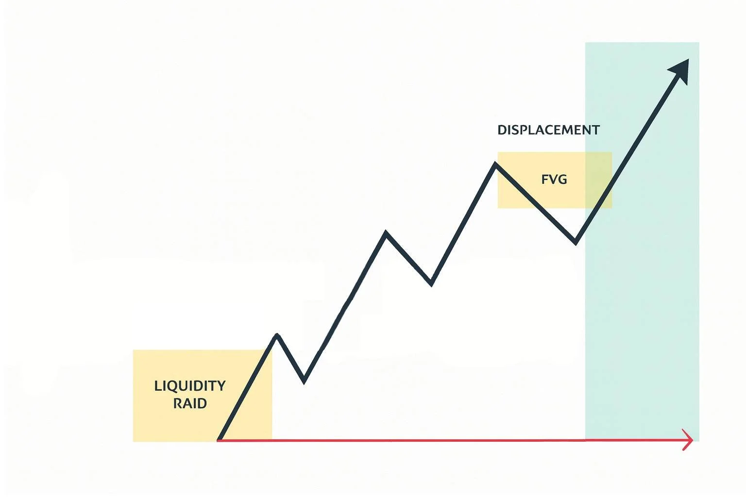
Step 1: The Liquidity Draw At the start of the window, identify the immediate "Draw on Liquidity." This is usually a distinct short-term High or Low that has formed just prior to the window or during the early minutes of the window. The algorithm seeks to run this level.

Step 2: The Raid and Displacement Price must sweep this liquidity level. Following the sweep, there must be an energetic reaction in the opposite direction—displacement. This is non-negotiable. The candle bodies must be large and decisive, indicating that the liquidity raid was a trap and smart money is now driving price the other way.

Step 3: The Fair Value Gap (FVG) The displacement leg must leave behind a Fair Value Gap (an inefficiency between three consecutive candles). This FVG is the entry signal. In the Silver Bullet model, the FVG is the trade.

Part 3: Execution and Management

The execution of the Silver Bullet is mechanical, designed to remove emotional decision-making.

Entry: The trader places a Limit Order at the edge of the Fair Value Gap formed inside the time window, or enters at Market upon a tap into the FVG.
Stop Loss: The stop is placed at the high/low of the displacement candle or, for a more conservative approach, beyond the swing high/low that caused the initial raid.
Take Profit: Because this is a low-latency, high-precision model, targets are often fixed or short-term. Common targets include the opposing liquidity pool (the nearest distinct high/low on the 1-minute or 5-minute chart) or a fixed risk-to-reward ratio (e.g., 2:1). Some traders use a fixed handle target (e.g., 10 points on ES/NASDAQ) to ensure consistency.

Part 4: Psychological and Strategic Advantages

The Silver Bullet acts as a forcing function for trader discipline. By ignoring price action for 21 hours of the day and hyper-focusing on these three specific hours, the trader avoids "death by a thousand cuts"—the common error of overtrading during low-probability choppy environments.

Furthermore, this model capitalizes on the "fractal" nature of markets. It does not require the daily chart to be trending beautifully; it only requires that within that 60-minute macro, the algorithm needs to move price from point A (liquidity pool) to point B (inefficiency). This makes the Silver Bullet highly effective even in range-bound market conditions where trend-following models might fail. It transforms trading from a game of prediction into a game of scheduled appointments with price.

Chapter 4 — ICT 2022 Mentorship Model

“Stop Hunt → MSS → PD Array Entry in Discount/Premium”

Introduction: The Algorithmic Simplification of Smart Money

The 2022 Mentorship Model represents the culmination of years of institutional theory distilled into a singular, highly structured, and almost algorithmic workflow. While previous iterations of ICT concepts required a broad synthesis of numerous variables, the 2022 Model formalizes the trade process into a rigorous checklist-driven strategy. It eliminates subjectivity by imposing a strict hierarchy of events: a liquidity raid must occur, followed by a confirmed structural shift, followed by a retracement into a specific valuation zone. This model operates on the premise that the market algorithm seeks two things: liquidity (stops) and inefficiencies (Fair Value Gaps). By waiting for the intersection of these two elements, the trader reduces the frequency of trades to focus exclusively on high-probability setups where institutional sponsorship is undeniable.

Part 1: The Context — Higher Timeframe Bias and Liquidity Mapping

The model begins long before the entry signal forms. It starts with a comprehensive assessment of the Higher Timeframe (HTF) Draw on Liquidity. Using Daily and Weekly charts, the trader must determine where price is ultimately being pulled. Is the market gravitating toward an unfinished weekly imbalance? Is it seeking to take out a monthly high? Without this magnetic heading, intraday setups are prone to failure. Once the destination is established, the trader maps the intraday liquidity pools that stand in the way. These include the highs and lows of the Asian session, previous session highs, and short-term swing points formed during the pre-market. The trader then adopts a posture of patience, waiting—often for hours—for price to interact with these levels.

Part 2: The Stop Hunt — The Mandatory Manipulation

The catalyst for the trade is the Stop Hunt (or Liquidity Raid). The price must stab through one of the identified liquidity pools in the direction opposite to the daily bias. If the bias is bullish, the trader waits for a violent dip below an old low; if bearish, a spike above an old high. This movement is the manipulation phase, designed to harvest stop-losses and induce retail traders into the wrong side of the market. Crucially, the 2022 Model dictates that this raid is mandatory. If price simply drifts toward the target without first engaging in a stop hunt to engineer liquidity, the setup is considered invalid. The algorithm requires fuel to move price; the stop hunt provides that fuel.

Part 3: The Market Structure Shift (MSS) and Displacement

Immediately following the raid, the trader drops to a lower timeframe—typically the 5-minute, 4-minute, or 3-minute chart—to identify the confirmation signal. This signal is the Market Structure Shift (MSS). An MSS occurs when price reverses from the stop hunt with significant energy, breaking a key internal swing point that supported the manipulation leg. This break must be accompanied by Displacement—a series of energetic candles with large bodies and short wicks, indicating a surge in institutional volume. If the break of structure is lethargic or wicky, it is discarded. The displacement is the "signature" of the smart money reversing their position after the liquidity grab.

Part 4: The Filter — Premium and Discount Arrays

What separates the 2022 Model from a generic reversal strategy is the strict application of Valuation. Once the displacement leg is established, the trader projects a Fibonacci grid (or simple 50% equilibrium tool) over the range of the move. The rules of institutional pricing dictate that smart money will only buy in a "Discount" (the lower 50% of the range) and will only sell in a "Premium" (the upper 50% of the range).

The trader then identifies the PD Arrays—specifically Fair Value Gaps (FVGs)—that exist within the displacement leg. However, only the arrays that sit in the correct valuation zone are valid. If a bullish FVG forms but it is located in the Premium (top half) of the leg, it is ignored because institutions will not buy expensive assets. The trader waits for price to retrace deep into the Discount zone to tag an FVG or Order Block. This filter drastically reduces premature entries and aligns the trader with the algorithmic pricing model used by interbank delivery engines.

Part 5: Execution and Discipline

The entry is taken as a limit order at the boundary of the Discount/Premium PD Array, with a stop loss placed safely beyond the swing point formed during the stop hunt. The target is the opposing liquidity pool or the Higher Timeframe draw identified in step one. This model teaches discipline above all else. If any element is missing—no liquidity sweep, no displacement, no MSS, or no PD array in the correct valuation zone—the setup is scrubbed. This selective process forces the trader to act like a sniper rather than a machine gunner, waiting for the perfect alignment of time, price, and structure.

Chapter 5 — Breaker Blocks and Continuation Models

The Role Reversal of Order Flow Structures

Introduction: When Old Support and Resistance Fail and Flip

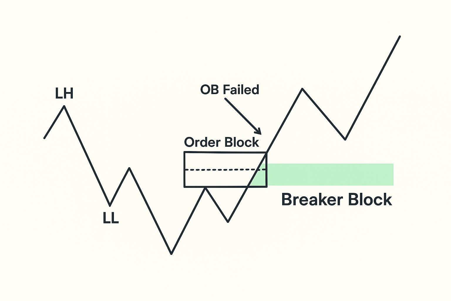
While Order Blocks (OBs) represent the definitive origin of institutional displacement, Breaker Blocks detail a more nuanced and tactical structure that emerges after a failed mitigation attempt. A Breaker Block is essentially a complex Order Block that was initially respected, later failed, and subsequently utilized as a structural pivot after a deeper liquidity raid. They are fundamental in understanding when the market has intentionally extended a move to gather more fuel before committing to the true directional delivery. This structure helps traders recognize not just the initial turning point, but reliable points of re-entry as the newly established trend unfolds. The logic hinges on the institutional necessity to acquire sufficient liquidity; if the first attempt at the Order Block fails to provide enough counterparty flow, the price must be driven deeper into an opposing liquidity pool before the genuine directional move can commence.

Part 1: The Anatomy and Logic of a Breaker Block

A typical Bullish Breaker formation follows a clear sequence. Price first shows respect for a previous high or a Bullish Order Block, suggesting accumulation is underway. However, the market later breaks below this attempted accumulation zone to hunt deeper Sell-Side Liquidity (SSL). This move liquidates the early buyers and provides the large volume of sell orders necessary for institutions to complete their accumulation phase. Following this deeper raid, price reverses strongly upward with displacement, initiating a Market Structure Shift (MSS). The original swing high or the last down-close candle before the failed accumulation zone (which was subsequently broken through) now transforms into the Breaker Block. When price retraces, this Breaker Block is expected to act as strong support. The psychological logic is simple: the institutional orders placed at the initial (failed) OB were not fully filled; the deeper raid allowed for full accumulation, and the original zone is now revisited as an anchor for the continuing move.

Part 2: The Breaker in Continuation Models

Breaker Blocks form the foundation of Continuation Models because they confirm that the market has committed to a new direction following a major structural shift. Instead of attempting to catch the absolute Low of the Day (the initial reversal), continuation models allow traders to enter safely after the initial volatility has subsided and the new trend is validated. The strategy dictates that once the initial MSS and Displacement define the new trend, traders should look for retracements into stacked PD Arrays that form along the trend's path. These arrays often include:

Fair Value Gaps (FVGs): Unfilled inefficiencies acting as magnetic pullbacks.
Breaker Blocks: The structural failure points that flip their role from resistance to support (or vice-versa).
Balanced Price Ranges (BPRs): Zones where a Bullish FVG and a Bearish FVG overlap, indicating heavy algorithmic activity.

This approach is particularly valuable after major Higher-Timeframe (HTF) Shifts where the market is expected to trend for days or weeks. The continuation model ensures the trader stays aligned with the established trend, using the Breaker Block as a highly reliable, structurally validated zone for re-entry.

Chapter 6 — Liquidity Sweep Scalps and Micro-Setups

Compressing ICT Logic to the Smallest Timeframes

Introduction: Scaling Down the Institutional Blueprint

Liquidity Sweep Scalps, or Micro-Setups, represent the application of the entire ICT framework—Accumulation, Manipulation, Distribution, Displacement, and PD Arrays—compressed onto the lowest practical timeframes, such as the 1-minute and 5-minute charts. This is not a change in logic, but a change in scale. The market microstructure remains fractal: the large-scale Power of Three occurring over a week is mirrored by a micro Accumulation $\rightarrow$ Manipulation $\rightarrow$ Distribution sequence that unfolds in 30 minutes. These setups appeal to advanced traders who seek high frequency opportunities and exceptionally tight stop-losses, but they demand a level of precision and discipline far beyond the higher-timeframe models.

Part 1: The Execution of the Micro Sweep

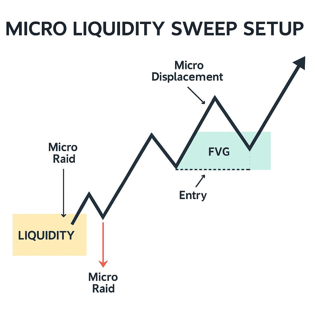
The process for executing a micro sweep is a time-compressed repetition of the core reversal model:

Micro Liquidity Identification: Identify small, obvious pools of liquidity on the 1-minute chart, often small equal highs or lows formed over the previous 15–30 minutes. These are the immediate targets for the scalp.
The Micro Raid: Wait for price to execute a sharp, quick raid of this liquidity. This typically happens with a single, fast candle wick that immediately pulls back.
Micro Displacement and FVG: Watch for immediate Displacement in the opposite direction, confirming the raid was a trap. This displacement must create a miniature Fair Value Gap (FVG) or a Micro Order Block (OB).
Entry and Target: Enter on the retracement back into the newly formed FVG/OB. Stop-losses are necessarily tight, placed just beyond the swing point of the raid. Targets are also scaled down, often the next small opposing liquidity pocket or a fixed, low-risk-to-reward objective (e.g., 1.5:1).

The principles are identical to the larger Liquidity Sweep Reversal Model (Chapter 1); only the magnitude of the move and the duration of the hold change.

Part 2: Precision, Noise, and Discipline

While conceptually simple, the practical execution of micro-setups demands significantly more precision and heightened emotional discipline. The low timeframes are heavily susceptible to noise, spread, and slippage, which can easily invalidate a trade with a stop-loss measured in only a few ticks. A trader attempting to navigate this environment must have an unshakeable grasp of the Higher Timeframe Bias; the micro-setup is only valid if it aligns with the direction of the 15-minute or 1-hour trend.

ICT repeatedly emphasizes a crucial caveat: Micro-setups are not for beginners. A trader must first master session-based models (like the Asia Range Raid) and reversal models (like the 2022 Mentorship Model) on higher timeframes before attempting these scalps. When approached with a validated core model understanding, micro sweep setups can yield exceptional precision and frequent opportunities, but they must be managed with a level of structure and risk management that matches their speed and volatility.

Chapter 7 — PD Array Hierarchy and Valuation

Institutional Reference Points and Order Block Logic

Introduction: The Language of Institutional Pricing

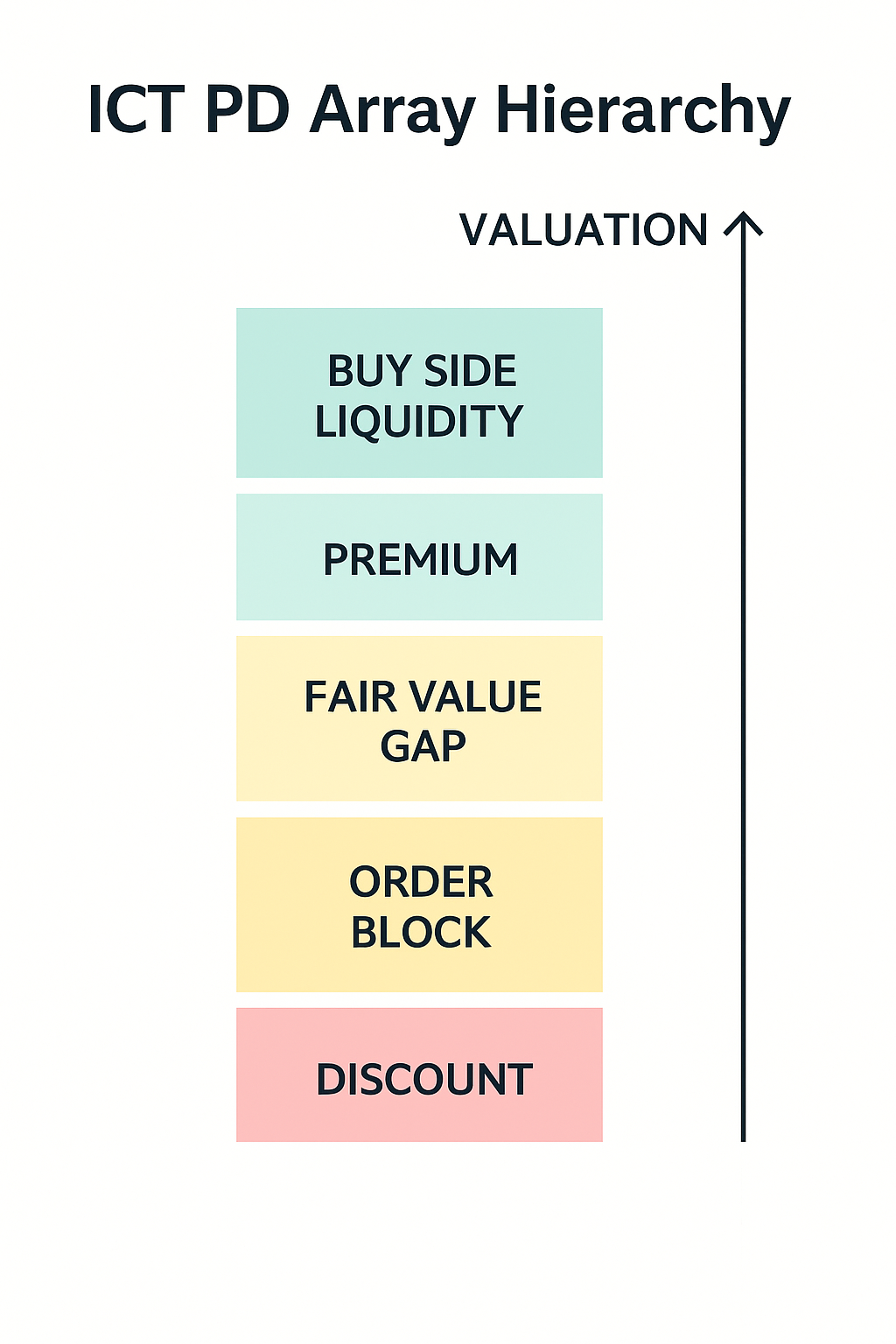
Within the ICT framework, PD Arrays (Price Delivery Arrays) are the specific institutional reference points where the market algorithm is expected to react, reverse, or consolidate. They are the footprints of institutional order flow and are essential for defining entry, stop-loss, and target levels. PD Arrays form a hierarchy based on their significance, with the ultimate filter for their use being the principle of Valuation—determining whether the price is currently in a Premium (expensive) or Discount (cheap) market. Understanding this hierarchy and filter is the key to high-probability execution.

Part 1: The Valuation Filter — Premium and Discount

Before engaging with any PD Array, a trader must first apply the Valuation Filter. Institutions will only buy assets when they are considered Discounted and only sell them when they are considered Premium. To determine valuation, the trader defines the price range (e.g., the daily range, a displacement leg, or a swing) and finds its Equilibrium (the midpoint or 50% level). The area above 50% is the Premium zone, where price is considered expensive, and PD arrays in this zone are only valid for Short entries. Conversely, the area below 50% is the Discount zone, where price is considered cheap, and PD arrays in this zone are only valid for Long entries. The most precise application of this concept is the Optimal Trade Entry (OTE), which typically refers to the 61.8% to 79% retracement levels within a price swing, representing the deepest discount or premium before expansion.

Part 2: The Core PD Array Hierarchy

PD Arrays are defined by their formation and intended institutional function. The most fundamental array is the Order Block (OB). An Order Block is the last up-close candle before a significant down move, or the last down-close candle before a significant up move, representing the point where large institutional orders were aggregated before the resultant displacement. When price returns to a Bullish OB (last down-close candle before the rally), it is anticipated to act as support; conversely, a Bearish OB (last up-close candle before the drop) is anticipated to act as resistance, as the remaining institutional orders are filled.

A second critical PD Array is the Fair Value Gap (FVG), also known as market inefficiency. This is a three-candle formation where the high of the first candle and the low of the third candle do not overlap with the second candle. This gap in price delivery indicates a swift, one-sided push. The market algorithm typically revisits these gaps to rebalance the orders, treating the FVG as a magnetic zone for retracement entries. A Bullish FVG is expected to act as support after a strong displacement up, while a Bearish FVG is expected to act as resistance after a strong displacement down.

The Role-Flipping Arrays

The Breaker Block is a more complex array representing a failed Order Block that subsequently flips its role. Breakers form when price attempts to accumulate at an OB, fails, pushes through for a deeper liquidity sweep, and then immediately reverses. The last opposing swing high/low that was broken becomes the Breaker. For a Bullish Breaker, the highest candle close in the accumulation area before the price drops to sweep liquidity is expected to act as support on the return. Breakers are instrumental in Continuation Models as they confirm that the market has committed to a new direction following a structural shift. Relatedly, a Mitigation Block forms when price returns to an Order Block, fails to reverse, and breaks through it entirely. The original Order Block then becomes a temporary anchor point for a continuation in the new direction. Mitigation Blocks are primarily used as a continuation reference after a shift in market structure, providing a zone for re-entry aligned with the new trend.

Part 3: Secondary PD Arrays

While the core arrays are used for entries, others provide valuable contextual information. Liquidity Voids are large gaps created by fast price movement, which are often filled quickly due to the market's tendency to reprice efficiently. A Balanced Price Range (BPR) is an area where a bullish FVG and a bearish FVG overlap, indicating a strong magnetic zone for consolidation or a reversal due to heavy algorithmic activity. Finally, Rejection Blocks are zones of strong, persistent wicking, which indicate institutional absorption or rejection of price at a specific level, highlighting a potential ceiling or floor.